Working on high performance computer such as the Massachusetts Green High Performance Computing Center (MGHPCC) requires a basic working knowledge of the Bash Unix shell and . On Ubuntu and Apple OSX computers, including the BCRC’s machine Bash is available through a program called Terminal. The terminal is also available within RStudio for Unix, OSX and Windows computers where we will use it from.
If you get “command not found” (or similar) when you try these steps through the RStudio terminal tab, you may need to set the type of terminal that gets launched by RStudio. Under some git install senerios, the git executable may not be available to the default terminal type. Follow the instructions on the RStudio site for Windows specific terminal options. In particular, you should choose “New Terminals open with Git Bash” in the Terminal options (Tools->Global Options->Terminal).
Like the R console where you can write R commands in the Bash shell/Terminal you can write shell commands. The terminal correlate of the .R file is the .sh file. You can open a new text file (File -> New File -> Text file) and save it as a .sh file. Like with R the hashtag is used to denote line that will not be run and for adding comments to your program. Similar to a .R file you can save a run a file with a batch of commands at the same time.
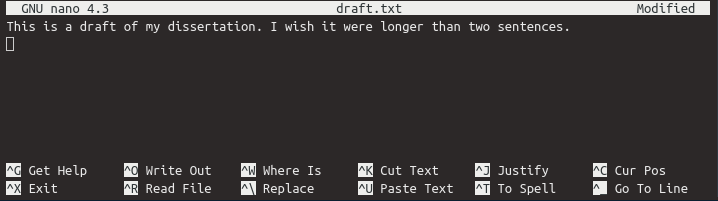
nano is a popular basic text editor that is called from the command line.
You can type in some text.
Once we’re happy with our text, we can press Ctrl+X (press the Ctrl or Control key and, while holding it down, press the X key) to write our data to disk (you’ll be asked to save the modified buffer. If you want to make the changes type Y)
To copy files.
To move a file
To delete my draft_old.txt change into that directory and using rm
Delete the MYDRAFT directory
Additional Resources
A less well-known fact about R Markdown is that many other languages are also supported, such as Python, Julia, C++, and SQL. The support comes from the knitr package, which has provided a large number of language engines. Language engines are essentially functions registered in the object knitr::knit_engine. You can list the names of all available engines via:
##  [1] "awk"       "bash"      "coffee"    "gawk"      "groovy"    "haskell"
##  [7] "lein"      "mysql"     "node"      "octave"    "perl"      "psql"
## [13] "Rscript"   "ruby"      "sas"       "scala"     "sed"       "sh"
## [19] "stata"     "zsh"       "highlight" "Rcpp"      "tikz"      "dot"
## [25] "c"         "fortran"   "fortran95" "asy"       "cat"       "asis"
## [31] "stan"      "block"     "block2"    "js"        "css"       "sql"
## [37] "go"        "python"    "julia"     "sass"      "scss"
You can run shell commands from within a RMarkdown file using ```{sh}… or {bash}…
Using sh or bash within RMarkdown has unusual quirk in that after a code chunk the working directory is reset to the original working directory where the .Rmd file is. This mean you have to be careful navigation to a new directory as in the above example to make sure all your commands are run in the same code chunk or you are likely to get an error.
In addition, because you will be creating and deleting files and directories you may want to set your {sh, eval = FALSE}... so that the commands are not run when you Knit.
There is a short nice introduction to Unix command line at Ohio Supercomputer Center that introduces the Unix commands cat, head, tail, chmod and grep that we will use in subsequent labs. Write a workflow that incorporates these commands plus the above pwd, cd, mkdir, ls, cp, mv and rm commands. You are free to borrow from the above examples, examples at the Ohio Super Computer Centero or other sites. Before doing this make a new empty folder on your computer, so that you don’t accidently modify or delete other files.
Put this workflow in a .sh file. When you are done put the steps with comments in .Rmd file with the {sh, eval=FALSE… and Knit. Turn in BOTH the .sh and .html files.
I am not sure all the Unix command with work on the Git Bash Terminal in Windows. If you any don’t please let me know.